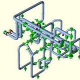
Mark a node (Node 10-Fig.2) at the location in the piping system where sway brace will be installed. Run Caesar analysis and note down the displacement of the point in specified direction from cold to operating condition. For the sake of example, let’s assume that CAESAR II calculated displacement from cold to operating position is 0.5 inch in +X direction.
Now in CAESAR II input spread sheet (See Fig. 2) check the restraints box and define bi-linear restraint (X2 for the assumed case) at Node 10 with CNode at 101. Here, K1 is the initial stiffness of a bi-linear restraint. Do not enter anything on this cell as the restraint is assumed to be rigid. The value of K2and Fy to be obtained from catalogue. Where, K2= Post yield stiffness of a bilinear restraint. When the load on the support restraint exceeds Fy then the stiffness on the support restraint changes from K1 to K2. Fy = Yield Load. If the load on the support restraint is less than “Fy” then the initial stiffness K1 is used. If the load on the support restraint is greater than “Fy” then the second stiffness ” K2″ is used.
Define restraint X at node 10 with CNode at 101. Provide a gap of 3 inch (=distance the sway brace is able to move in both positive and negative direction before it gets locked/ become fully rigid depending on manufacturer= 3 inch as per C&P catalogue)
Check the displacement box and define the displacement for Node 101. It is the displacement for node 10 as noted earlier (0.5 inch in X direction, leave other cells i.e., DY, DZ, RX, RY, RZ blank.).
Add D2 in sustained and operating load cases. Now run the analysis to obtain results.
Underground or buried piping are all piping which runs below grade. In every process industry there will be few lines (Sewer or drainage system, Sanitary and Storm Water lines, Fire water or drinking water lines etc), part of which normally runs underground. However the term buried piping or underground piping, in true sense, appears for pipeline industry as miles of long pipe run carrying fluids will be there.
Analyzing an underground pipe line is quite different from analyzing plant piping. Special problems are involved because of the unique characteristics of a pipeline, code requirements and techniques required in analysis. Elements of analysis include pipe movements, anchorage force, soil friction, lateral soil force and soil pipe interaction.
Analyzing an underground pipe line is quite different from analyzing plant piping. Special problems are involved because of the unique characteristics of a pipeline, code requirements and techniques required in analysis. Elements of analysis include pipe movements, anchorage force, soil friction, lateral soil force and soil pipe interaction.
To appreciate pipe code requirements and visualize problems involved in pipe line stress analysis, it is necessary to first distinguish a pipe line from plant piping. Unique characteristics of a pipe line include:
• High allowable stress: A pipe line has a rather simple shape. It is circular and very often runs several miles before making a turn. Therefore, the stresses calculated are all based on simple static equilibrium formulas which are very reliable. Since stresses produced are predictable, allowable stress used is considerable higher than that used in plant piping.
• High yield strength pipe: To raise the allowable, the first obstacle is yield strength. Although a pipe line operating beyond yield strength may not create structural integrity problems, it may cause undesirable excessive deformation and possibility of strain follow up. Therefore, high test line with a very high yield to ultimate strength ratio is normally used in pipe line construction. Yield strength in some pipe can be as high as 80 percent of ultimate strength. All allowable stresses are based only on yield strength.
• High pressure elongation: Movement of pipe line is normally due to expansion of a very long line at low temperature difference. Pressure elongation, negligible in plant piping, contributes much of the total movement and must be included in the analysis.
• Soil- pipe interaction: The main portion of a pipe line is buried underground. Any pipe movement has to overcome soil force, which can be divided into two categories: Friction force created from sliding and pressure force resulting from pushing. The major task of pipe line analysis is to investigate soil- pipe interaction which has never been a subject in plant piping analysis.
• High yield strength pipe: To raise the allowable, the first obstacle is yield strength. Although a pipe line operating beyond yield strength may not create structural integrity problems, it may cause undesirable excessive deformation and possibility of strain follow up. Therefore, high test line with a very high yield to ultimate strength ratio is normally used in pipe line construction. Yield strength in some pipe can be as high as 80 percent of ultimate strength. All allowable stresses are based only on yield strength.
• High pressure elongation: Movement of pipe line is normally due to expansion of a very long line at low temperature difference. Pressure elongation, negligible in plant piping, contributes much of the total movement and must be included in the analysis.
• Soil- pipe interaction: The main portion of a pipe line is buried underground. Any pipe movement has to overcome soil force, which can be divided into two categories: Friction force created from sliding and pressure force resulting from pushing. The major task of pipe line analysis is to investigate soil- pipe interaction which has never been a subject in plant piping analysis.
Normally this line does not have high design temperatures (of the order of 60 to 80 degree centigrade) and only thermal stress checking is sufficient for underground part. Common materials used for underground piping are Carbon Steel, Ductile iron, cast Iron, Stainless Steel and FRP/GRP.
I will try to explain the steps followed while analysing such systems using Caesar II. However this article does not cover the basic theory for analysis.
Inputs Required for Analysis:
Before proceeding for analysis of buried piping using Caesar II collect the following information from related department
1. Isometric drawings or GA drawings of the pipeline from Piping layout Department.
2. Line parameters (Temperature, Pressure, Material, Fluid Density, etc) from process Department.
3. Soil Properties from Civil Department.
Before proceeding for analysis of buried piping using Caesar II collect the following information from related department
1. Isometric drawings or GA drawings of the pipeline from Piping layout Department.
2. Line parameters (Temperature, Pressure, Material, Fluid Density, etc) from process Department.
3. Soil Properties from Civil Department.
Caesar II for Underground Piping Analysis:
The CAESAR II underground pipe modeler is designed to simplify user input of buried pipe data. To achieve this objective the “Modeler” performs the following functions for analyst:
• Allows the direct input of soil properties. The “Modeler” contains the equations for buried pipe stiffnesses that are outlined later in this report. These equations are used to calculate first the stiffnesses on a per length of pipe basis, and then generate the restraints that simulate the discrete buried pipe restraint.
• Breaks down straight and curved lengths of pipe to locate soil restraints. CAESAR II uses a zone concept to break down straight and curved sections. Where transverse bearing is a concern (near bends, tees, and entry/exit points), soil restraints are located in close proximity and where axial load dominates, soil restraints are spaced far apart.
• Allows the direct input of user-defined soil stiffnesses on a per length of pipe basis. Input parameters include axial, transverse, upward, and downward stiffnesses, as well as ultimate loads. Users can specify user-defined stiffnesses separately, or in conjunction with CAESAR II’s automatically generated soil stiffnesses.
The CAESAR II underground pipe modeler is designed to simplify user input of buried pipe data. To achieve this objective the “Modeler” performs the following functions for analyst:
• Allows the direct input of soil properties. The “Modeler” contains the equations for buried pipe stiffnesses that are outlined later in this report. These equations are used to calculate first the stiffnesses on a per length of pipe basis, and then generate the restraints that simulate the discrete buried pipe restraint.
• Breaks down straight and curved lengths of pipe to locate soil restraints. CAESAR II uses a zone concept to break down straight and curved sections. Where transverse bearing is a concern (near bends, tees, and entry/exit points), soil restraints are located in close proximity and where axial load dominates, soil restraints are spaced far apart.
• Allows the direct input of user-defined soil stiffnesses on a per length of pipe basis. Input parameters include axial, transverse, upward, and downward stiffnesses, as well as ultimate loads. Users can specify user-defined stiffnesses separately, or in conjunction with CAESAR II’s automatically generated soil stiffnesses.
Modeling steps followed in Caesar II:
The modeling of buried piping is very easy if you have all the data at your hand. The following steps are followed for modeling:
The modeling of buried piping is very easy if you have all the data at your hand. The following steps are followed for modeling:
• From the isometric model the line in the same way as you follow in case of above ground pipe model i.e, enter line properties in Caesar Spreadsheet, enter lengths by breaking the line into several nodes or select an existing job for converting it into an underground model.
• Analyst can start the Buried Pipe Modeler by selecting an existing job and then choosing Input-Underground from the CAESAR II Main Menu. The Modeler is designed to read a standard CAESAR II input data file that describes the basic layout of the piping system as if it was not buried. From this basic input CAESAR II creates a second input data file that contains the buried pipe model. This second input file typically contains a much larger number of elements and restraints than the first job. The first job that serves as the “pattern” is termed the original job. The second file that contains the element mesh refinement and the buried pipe restraints is termed the buried job. CAESAR II names the buried job by appending a “B” to the name of the original job.
• When the Buried Pipe Modeler is initially started up, the following screen appears:
• Analyst can start the Buried Pipe Modeler by selecting an existing job and then choosing Input-Underground from the CAESAR II Main Menu. The Modeler is designed to read a standard CAESAR II input data file that describes the basic layout of the piping system as if it was not buried. From this basic input CAESAR II creates a second input data file that contains the buried pipe model. This second input file typically contains a much larger number of elements and restraints than the first job. The first job that serves as the “pattern” is termed the original job. The second file that contains the element mesh refinement and the buried pipe restraints is termed the buried job. CAESAR II names the buried job by appending a “B” to the name of the original job.
• When the Buried Pipe Modeler is initially started up, the following screen appears:
This spreadsheet is used to enter the buried element descriptions for the job. The buried element description spreadsheet serves several functions:
• Allows analyst to define which part of the piping system is buried.
• Allows analyst to define mesh spacing at specific element ends.
• Allows the input of user-defined soil stiffnesses.
From/ To node:-
Any element of pipe in CAESAR II can be define by two elements first is start point and second is end point. In buried pipe model, before conversion the From/ To nodes remains same as unburied model.
• Allows analyst to define which part of the piping system is buried.
• Allows analyst to define mesh spacing at specific element ends.
• Allows the input of user-defined soil stiffnesses.
From/ To node:-
Any element of pipe in CAESAR II can be define by two elements first is start point and second is end point. In buried pipe model, before conversion the From/ To nodes remains same as unburied model.