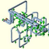
Basics for Fatigue Analysis of Piping System using Caesar II ⬇️
Fatigue is the progressive and localized structural damage that occurs when a material is subjected to cyclic loading. Continued cycling of high stress concentrations may eventually cause a crack which propagates and results in leakages. This failure mechanism is called fatigue. Damage once done during the fatigue process is cumulative and normally unrecoverable.
Fatigue can be grouped in two classes; High cycle fatigue and low cycle fatigue.
High cycle fatigue involves little or no plastic action. Therefore, it is stress-governed. Normally, a fatigue curve (also called the S–N curve) is generated for every material by experimental tests which correlates applied stress with the number of cycles to cause failure. For high-cycle fatigue, the analysis is performed to determine the endurance limit, which is actually a stress level that can be applied for an infinite number of times without showing any failure. As a general rule no of cycles 10^5 is considered as demarcation point for high and low cycle fatigue.
Fatigue can be grouped in two classes; High cycle fatigue and low cycle fatigue.
High cycle fatigue involves little or no plastic action. Therefore, it is stress-governed. Normally, a fatigue curve (also called the S–N curve) is generated for every material by experimental tests which correlates applied stress with the number of cycles to cause failure. For high-cycle fatigue, the analysis is performed to determine the endurance limit, which is actually a stress level that can be applied for an infinite number of times without showing any failure. As a general rule no of cycles 10^5 is considered as demarcation point for high and low cycle fatigue.
The loading cycles applied in piping design are normally very few in the order of a few thousands. This type of fatigue is identified as low-cycle fatigue. For low-cycle fatigue, the applied stress normally exceeds the yield strength of the material, which causes plastic instability in the specimen under test. But when strain is used as the controlled variable, the results in low-cycle region are reliable as well as reproducible.
Sources of Fatigue:⬇️⬇️
For Piping system, Cyclic loadings are primarily due to:
* Thermal Expansion & Contraction
* Vibration due to Occasional loading
* Pressure variation within Piping system
* Motion wave.
* Due to Flow induced Vibration
The fatigue process is divided into three stages: crack initiation from the continued cycling of high stress concentrations, crack propagation to critical size, and unstable rupture of the section.
For Piping system, Cyclic loadings are primarily due to:
* Thermal Expansion & Contraction
* Vibration due to Occasional loading
* Pressure variation within Piping system
* Motion wave.
* Due to Flow induced Vibration
The fatigue process is divided into three stages: crack initiation from the continued cycling of high stress concentrations, crack propagation to critical size, and unstable rupture of the section.
Factors Affecting the Fatigue Behavior:⬇️⬇️⬇️
The factors which affect the fatigue behaviour are listed below:
*Type and Nature of Loading.
*Size of Component and stress or strain Distribution.
* Surface finish and Directional Properties.
*Stress or Strain Concentration.
*Mean stress or Strain.
*Environmental Effects.
*Metallurgical Factors and Material Properties.
*Strain Rate and Frequency Effects.
The factors which affect the fatigue behaviour are listed below:
*Type and Nature of Loading.
*Size of Component and stress or strain Distribution.
* Surface finish and Directional Properties.
*Stress or Strain Concentration.
*Mean stress or Strain.
*Environmental Effects.
*Metallurgical Factors and Material Properties.
*Strain Rate and Frequency Effects.
Characteristics of Low Cycle Fatigue:⬇️⬇️⬇️⬇️
*Characterized by high loads and a small no. of cycles before failure.
*Here failure occurs only with stress levels in the plastic range, i.e. significant plastic strain occurs during each cycle.
*The stresses which cause fatigue failure in the piping are the peak stresses.
*In piping design, most of the loading cycles encountered would be of the low cycle type
*Characterized by high loads and a small no. of cycles before failure.
*Here failure occurs only with stress levels in the plastic range, i.e. significant plastic strain occurs during each cycle.
*The stresses which cause fatigue failure in the piping are the peak stresses.
*In piping design, most of the loading cycles encountered would be of the low cycle type
Characteristics of High Cycle Fatigue:⬇️⬇️⬇️⬇️⬇️
*Characterized by high no. of cycles (Preferable N>10^4) with relatively low stress levels and the deformation is in elastic range.
*This type of fatigue failure used in the design of rotating machinery.
*This type of fatigue results from strain cycles in the elastic range.
*A stress level, endurance limit, may be applied an infinite times without failure, is calculated.
*Characterized by high no. of cycles (Preferable N>10^4) with relatively low stress levels and the deformation is in elastic range.
*This type of fatigue failure used in the design of rotating machinery.
*This type of fatigue results from strain cycles in the elastic range.
*A stress level, endurance limit, may be applied an infinite times without failure, is calculated.
Failure Criteria:⬇️
While preparing fatigue curves, the strains obtained in the tests are multiplied by one-half of the elastic modulus to obtain pseudo stress amplitude. This pseudo stress is directly compared with the stresses calculated on the assumption of elastic behavior of piping. During piping stress analysis, a stress called the alternating stress (Salt) is used which is defined as one-half of the calculated peak stress. Fatigue failure can be prevented by ensuring that the number of load cycles (N) associated with a specific alternating stress is less than the number allowed in the S–N curve or endurance curve. But in practical service conditions a piping system is subjected to alternating stresses of different magnitudes. These changes in magnitudes make the direct use of the fatigue curves inapplicable since the curves are based on constant-stress amplitude.
Fatigue tests of metallic materials and structures have provided the following main clues to the basic nature of fatigue:
* Fatigue failure, or cracking under repeated stress much lower than the ultimate tensile strength, is shown in most metals and alloys that exhibit some ductility in static tests. The magnitude of the applied alternating stress range is the controlling fatigue life parameter.
* Failure depends upon the number of repetitions of a given range of stress rather than the total time under load. The speed of loading is a factor of secondary importance, except at elevated temperatures.
* Some metals, including ferrous alloys, have a safe range of stress. Below this stress, called the “endurance limit or fatigue limit”, failure does not occur irrespective of the number of stress cycles.
* Notches, grooves, or other discontinuities of section greatly decrease the stress amplitude that can be sustained for a given number of cycles.
* The range of stress necessary to produce failure in a fixed number of cycles usually decrease as the mean tension stress of the loading cycle is increased.
* Examination of fatigue fracture shows evidence of microscopic deformation, ever in the apparently brittle region of origin and propagates of the crack. The plastic deformation that accompanies a spreading fatigue crack is usually limited in extent to regions very near the crack.
Therefore, to make fatigue curves applicable for piping, some alternate approach is necessary.
One hypothesis asserts that the damage fraction of any stress level S, is linearly proportional to the Ratio of the number of cycles of operation at the stress level to the total number of cycles that would produce failure at that stress level. This means that failure is predicted to occur if U≥1.0 where U= Usage factor = ∑(ni/Ni) for all stress levels Where, ni= number of cycles operating at stress level i , Ni= number of cycles to failure at stress level i as per material fatigue curve.
While preparing fatigue curves, the strains obtained in the tests are multiplied by one-half of the elastic modulus to obtain pseudo stress amplitude. This pseudo stress is directly compared with the stresses calculated on the assumption of elastic behavior of piping. During piping stress analysis, a stress called the alternating stress (Salt) is used which is defined as one-half of the calculated peak stress. Fatigue failure can be prevented by ensuring that the number of load cycles (N) associated with a specific alternating stress is less than the number allowed in the S–N curve or endurance curve. But in practical service conditions a piping system is subjected to alternating stresses of different magnitudes. These changes in magnitudes make the direct use of the fatigue curves inapplicable since the curves are based on constant-stress amplitude.
Fatigue tests of metallic materials and structures have provided the following main clues to the basic nature of fatigue:
* Fatigue failure, or cracking under repeated stress much lower than the ultimate tensile strength, is shown in most metals and alloys that exhibit some ductility in static tests. The magnitude of the applied alternating stress range is the controlling fatigue life parameter.
* Failure depends upon the number of repetitions of a given range of stress rather than the total time under load. The speed of loading is a factor of secondary importance, except at elevated temperatures.
* Some metals, including ferrous alloys, have a safe range of stress. Below this stress, called the “endurance limit or fatigue limit”, failure does not occur irrespective of the number of stress cycles.
* Notches, grooves, or other discontinuities of section greatly decrease the stress amplitude that can be sustained for a given number of cycles.
* The range of stress necessary to produce failure in a fixed number of cycles usually decrease as the mean tension stress of the loading cycle is increased.
* Examination of fatigue fracture shows evidence of microscopic deformation, ever in the apparently brittle region of origin and propagates of the crack. The plastic deformation that accompanies a spreading fatigue crack is usually limited in extent to regions very near the crack.
Therefore, to make fatigue curves applicable for piping, some alternate approach is necessary.
One hypothesis asserts that the damage fraction of any stress level S, is linearly proportional to the Ratio of the number of cycles of operation at the stress level to the total number of cycles that would produce failure at that stress level. This means that failure is predicted to occur if U≥1.0 where U= Usage factor = ∑(ni/Ni) for all stress levels Where, ni= number of cycles operating at stress level i , Ni= number of cycles to failure at stress level i as per material fatigue curve.
Analysis Requirement:⬇️⬇️
If there are two or more types of stress cycles which produce significant stresses, their cumulative effect shall be evaluated as stipulated in Steps 1 through 6 below:
1- Designate the specified number of times each type of stress cycle of types 1,2,3,…,n, will be Repeated during the life of the component as n1, n2, n3,……., nn, respectively. In determining n1, n2, n3,……., nn, consideration shall be given to the superposition of cycles of various origins which produce the greatest total alternating stress range. For example , if one type of stress cycle produce 1000 cycles of a stress variation from zero to +60,000 psi and another type of stress cycle produces 10,000 cycles of a stress variation from zero to -50,000 psi, the two cycles to be considered are shown below:
* cycle type 1: n1=1000 and Salt1= (60000+50000)/2
* cycle type 2: n2=9000 and Salt2= (0+50000)/2
* For each type of stress cycle, determine the alternating stress intensity Salt, which for our application is one half of the range between the expansion stress cycles (as shown above). These alternating stress intensities are designated as Salt1, Salt2, Saltn.
* On the applicable design fatigue curve find the permissible number of cycles for each Salt computed. These are designated as N1, N2, …….Nn.
* For each stress cycle calculate the usage factor U1, U2, …….Un where U1= n1/N1, U2= n2/N2,……..Un=nn/Nn.
* Calculate the cumulative usage factor U as U=U1+U2+…….+Un.
* The cumulative usage factor shall not exceed 1.0
If there are two or more types of stress cycles which produce significant stresses, their cumulative effect shall be evaluated as stipulated in Steps 1 through 6 below:
1- Designate the specified number of times each type of stress cycle of types 1,2,3,…,n, will be Repeated during the life of the component as n1, n2, n3,……., nn, respectively. In determining n1, n2, n3,……., nn, consideration shall be given to the superposition of cycles of various origins which produce the greatest total alternating stress range. For example , if one type of stress cycle produce 1000 cycles of a stress variation from zero to +60,000 psi and another type of stress cycle produces 10,000 cycles of a stress variation from zero to -50,000 psi, the two cycles to be considered are shown below:
* cycle type 1: n1=1000 and Salt1= (60000+50000)/2
* cycle type 2: n2=9000 and Salt2= (0+50000)/2
* For each type of stress cycle, determine the alternating stress intensity Salt, which for our application is one half of the range between the expansion stress cycles (as shown above). These alternating stress intensities are designated as Salt1, Salt2, Saltn.
* On the applicable design fatigue curve find the permissible number of cycles for each Salt computed. These are designated as N1, N2, …….Nn.
* For each stress cycle calculate the usage factor U1, U2, …….Un where U1= n1/N1, U2= n2/N2,……..Un=nn/Nn.
* Calculate the cumulative usage factor U as U=U1+U2+…….+Un.
* The cumulative usage factor shall not exceed 1.0
Pressure Testing ⬇️
Catastrophic failure during Hydro testing
This incident occurred 4 May 2011 on a pipeline project during a hydro-test of new piping.
The fabrication, consisting of 24in schedule 30 pipe & fittings, was in the process of being hydro-tested when the failure occurred. There was approximately 80 linear feet of piping included in the test. The piping was to be pressurized to 149 bar. When the test pressure reached 120 bar, there was a loud noise, similar to a gunshot.
Catastrophic failure during Hydro testing
This incident occurred 4 May 2011 on a pipeline project during a hydro-test of new piping.
The fabrication, consisting of 24in schedule 30 pipe & fittings, was in the process of being hydro-tested when the failure occurred. There was approximately 80 linear feet of piping included in the test. The piping was to be pressurized to 149 bar. When the test pressure reached 120 bar, there was a loud noise, similar to a gunshot.
Modal Frequency checking Method (Modal Analysis) using Caesar II ⬇️
While performing stress analysis for process piping you might have come across the term two phase flow. The stress analysis basis or flexibility specification of most of the relevant organization informs the stress engineers to properly support these lines using hold-downs, guides and axial stops. The main reason is that two phase flow lines are vibration prone lines. Many organizations prefer to keep the natural frequency of those lines in excess of 4 Hz to reduce the possibility of vibration. Now the question is how to calculate the natural frequency of the complex piping system?
There comes the importance of a Caesar II dynamic module called Modal analysis module. The complex job of calculating the natural frequency of the piping system becomes very easy with the use of this module. The vibration response or dynamic response of any system can be easily determined using modal analysis. In actual case, Modal analysis breaks up a complex system into a number of modes of vibration, each of which is having a unique vibration response. This article will elaborate the steps followed for performing modal analysis module using Caesar II.
There comes the importance of a Caesar II dynamic module called Modal analysis module. The complex job of calculating the natural frequency of the piping system becomes very easy with the use of this module. The vibration response or dynamic response of any system can be easily determined using modal analysis. In actual case, Modal analysis breaks up a complex system into a number of modes of vibration, each of which is having a unique vibration response. This article will elaborate the steps followed for performing modal analysis module using Caesar II.
To start the modal analysis you must have a stress system. So from isometric model the system following conventional methods and perform the static analysis and make the system safe in all respect with respect to static analysis. Now follow the below mentioned steps for dynamic Modal analysis.
* Click on Analysis-Dynamic Analysis as shown in Fig. 1 to open the dynamic module in Caesar II. It will open the window which is shown in Fig. 2.
* Click on Analysis-Dynamic Analysis as shown in Fig. 1 to open the dynamic module in Caesar II. It will open the window which is shown in Fig. 2.